Kinked beam

Kinked beam#

Attention

This page shows a preview of the assignment. Please fork and clone the assignment to work on it locally from GitHub

Added in version v2025.2.0: After workshop 2

Solutions additional assignments in text and downloads

Given is the following beam [HansWfDUoTechnology22]:

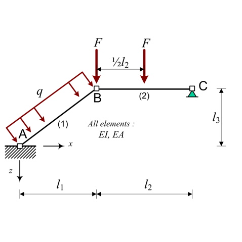
https://raw.githubusercontent.com/ibcmrocha/public/main/newforce.png

With:

\(l_1 = 4\)
\(l_2 = 5\)
\(l_3 = 3\)
\(EI = 5000\)
\(EA = 15000\)
\(q = 6\)
\(F = 40\)

Exercise (Kinked beam)

Solve this problem.

import matplotlib as plt
import numpy as np
sys.path.insert(1, '/matrixmethod_solution')
import matrixmethod_solution as mm
%config InlineBackend.figure_formats = ['svg']

import numpy as np
import matplotlib as plt
import matrixmethod as mm
%config InlineBackend.figure_formats = ['svg']

#YOUR_CODE_HERE

Solution to Exercise (Kinked beam)

This problem could be solved without any additional coding by adding an additional node at the points load halfway beam (2)
Another options is to add an element with a concentrated load at midspan. This option is chosen here.

import sympy as sym

import sympy as sym
sym.init_printing()

EI, F, x = sym.symbols('EI, F, x')
L = sym.symbols('L',positive=True)
w = sym.Function('w')

ODE_bending = sym.Eq(w(x).diff(x, 4) *EI, F*sym.SingularityFunction(x, L/2, -1))
display(ODE_bending)

V = - sym.integrate(ODE_bending.rhs, x) + sym.symbols('C1')
M = sym.integrate(V, x) + sym.symbols('C2')
kappa = M / EI
phi = sym.integrate(kappa, x) + sym.symbols('C3')
w = -sym.integrate(phi, x) + sym.symbols('C4')
display(w)

w_1, w_2, phi_1, phi_2 = sym.symbols('w_1, w_2, phi_1, phi_2')
phi = -w.diff(x)
eq1 = sym.Eq(w.subs(x,0),w_1)
eq2 = sym.Eq(w.subs(x,L),w_2)
eq3 = sym.Eq(phi.subs(x,0),phi_1)
eq4 = sym.Eq(phi.subs(x,L),phi_2)
C_sol = sym.solve([eq1, eq2, eq3, eq4 ], sym.symbols('C1, C2, C3, C4'))
for key in C_sol:
    display(sym.Eq(key, C_sol[key]))

display(sym.collect(M.subs(C_sol).expand(),[w_1,w_2,phi_1,phi_2, F]))
display(sym.collect(w.subs(C_sol).expand(),[w_1,w_2,phi_1,phi_2, F]))

F_1_z, F_2_z, T_1_y, T_2_y = sym.symbols('F_1_z, F_2_z, T_1_y, T_2_y')

eq5 = sym.Eq(-V.subs(C_sol).subs(x,0), F_1_z)
eq6 = sym.Eq(V.subs(C_sol).subs(x,L), F_2_z)
eq7 = sym.Eq(-M.subs(C_sol).subs(x,0), T_1_y)
eq8 = sym.Eq(M.subs(C_sol).subs(x,L), T_2_y)
display(eq5, eq6, eq7, eq8)

A, b = sym.linear_eq_to_matrix([eq5,eq7, eq6, eq8], [w_1, phi_1, w_2, phi_2])
display(A,b)

\[\displaystyle EI \frac{d^{4}}{d x^{4}} w{\left(x \right)} = F {\left\langle - \frac{L}{2} + x \right\rangle}^{-1}\]

\[\displaystyle - C_{3} x + C_{4} - \frac{\frac{C_{1} x^{3}}{6} + \frac{C_{2} x^{2}}{2} - \frac{F {\left\langle - \frac{L}{2} + x \right\rangle}^{3}}{6}}{EI}\]

\[\displaystyle C_{1} = \frac{12 EI L \phi_{1} + 12 EI L \phi_{2} - 24 EI w_{1} + 24 EI w_{2} + F L^{3}}{2 L^{3}}\]

\[\displaystyle C_{2} = \frac{- 32 EI L \phi_{1} - 16 EI L \phi_{2} + 48 EI w_{1} - 48 EI w_{2} - F L^{3}}{8 L^{2}}\]

\[\displaystyle C_{3} = \phi_{1}\]

\[\displaystyle C_{4} = w_{1}\]

\[\displaystyle F \left(- \frac{L}{8} + \frac{x}{2} - {\left\langle - \frac{L}{2} + x \right\rangle}^{1}\right) + \phi_{1} \left(- \frac{4 EI}{L} + \frac{6 EI x}{L^{2}}\right) + \phi_{2} \left(- \frac{2 EI}{L} + \frac{6 EI x}{L^{2}}\right) + w_{1} \cdot \left(\frac{6 EI}{L^{2}} - \frac{12 EI x}{L^{3}}\right) + w_{2} \left(- \frac{6 EI}{L^{2}} + \frac{12 EI x}{L^{3}}\right)\]

\[\displaystyle F \left(\frac{L x^{2}}{16 EI} - \frac{x^{3}}{12 EI} + \frac{{\left\langle - \frac{L}{2} + x \right\rangle}^{3}}{6 EI}\right) + \phi_{1} \left(- x + \frac{2 x^{2}}{L} - \frac{x^{3}}{L^{2}}\right) + \phi_{2} \left(\frac{x^{2}}{L} - \frac{x^{3}}{L^{2}}\right) + w_{1} \cdot \left(1 - \frac{3 x^{2}}{L^{2}} + \frac{2 x^{3}}{L^{3}}\right) + w_{2} \cdot \left(\frac{3 x^{2}}{L^{2}} - \frac{2 x^{3}}{L^{3}}\right)\]

\[\displaystyle - \frac{12 EI L \phi_{1} + 12 EI L \phi_{2} - 24 EI w_{1} + 24 EI w_{2} + F L^{3}}{2 L^{3}} = F_{1 z}\]

\[\displaystyle - F + \frac{12 EI L \phi_{1} + 12 EI L \phi_{2} - 24 EI w_{1} + 24 EI w_{2} + F L^{3}}{2 L^{3}} = F_{2 z}\]

\[\displaystyle - \frac{- 32 EI L \phi_{1} - 16 EI L \phi_{2} + 48 EI w_{1} - 48 EI w_{2} - F L^{3}}{8 L^{2}} = T_{1 y}\]

\[\displaystyle - \frac{F L}{2} + \frac{- 32 EI L \phi_{1} - 16 EI L \phi_{2} + 48 EI w_{1} - 48 EI w_{2} - F L^{3}}{8 L^{2}} + \frac{12 EI L \phi_{1} + 12 EI L \phi_{2} - 24 EI w_{1} + 24 EI w_{2} + F L^{3}}{2 L^{2}} = T_{2 y}\]

\[\begin{split}\displaystyle \left[\begin{matrix}\frac{12 EI}{L^{3}} & - \frac{6 EI}{L^{2}} & - \frac{12 EI}{L^{3}} & - \frac{6 EI}{L^{2}}\\- \frac{6 EI}{L^{2}} & \frac{4 EI}{L} & \frac{6 EI}{L^{2}} & \frac{2 EI}{L}\\- \frac{12 EI}{L^{3}} & \frac{6 EI}{L^{2}} & \frac{12 EI}{L^{3}} & \frac{6 EI}{L^{2}}\\- \frac{6 EI}{L^{2}} & \frac{2 EI}{L} & \frac{6 EI}{L^{2}} & \frac{4 EI}{L}\end{matrix}\right]\end{split}\]

\[\begin{split}\displaystyle \left[\begin{matrix}\frac{F}{2} + F_{1 z}\\- \frac{F L}{8} + T_{1 y}\\\frac{F}{2} + F_{2 z}\\\frac{F L}{8} + T_{2 y}\end{matrix}\right]\end{split}\]

So, the load vector is: \(\left[\begin{matrix}\frac{F}{2}\\- \frac{F L}{8}\\\frac{F}{2}\\\frac{F L}{8}\end{matrix}\right]\)
The new expression for M is: \(- \frac{F L}{8} + \frac{F x}{2} - F \left(\begin{cases} - \frac{L}{2} + x & \text{for}\: x > \frac{L}{2} \\0 & \text{otherwise} \end{cases}\right) + \phi_{1} \left(- \frac{4 EI}{L} + \frac{6 EI x}{L^{2}}\right) + \phi_{2} \left(- \frac{2 EI}{L} + \frac{6 EI x}{L^{2}}\right) + w_{1} \cdot \left(\frac{6 EI}{L^{2}} - \frac{12 EI x}{L^{3}}\right) + w_{2} \left(- \frac{6 EI}{L^{2}} + \frac{12 EI x}{L^{3}}\right)\)
The new expression for w is: \(\phi_{1} \left(- x + \frac{2 x^{2}}{L} - \frac{x^{3}}{L^{2}}\right) + \phi_{2} \left(\frac{x^{2}}{L} - \frac{x^{3}}{L^{2}}\right) + w_{1} \cdot \left(1 - \frac{3 x^{2}}{L^{2}} + \frac{2 x^{3}}{L^{3}}\right) + w_{2} \cdot \left(\frac{3 x^{2}}{L^{2}} - \frac{2 x^{3}}{L^{3}}\right) + \frac{F L x^{2}}{16 EI} - \frac{F x^{3}}{12 EI} + \frac{F \left(\begin{cases} \left(- \frac{L}{2} + x\right)^{3} & \text{for}\: x > \frac{L}{2} \\0 & \text{otherwise} \end{cases}\right)}{6 EI}\)
These changes have been implemented in the EB_point_load_element class in ./matrixmethod/elements.py.

mm.Node.clear()
mm.Element.clear()

l1 = 4
l2 = 5
l3 = 3
EI = 5000
q = 6
F = 40
EA = 15000

nodes = []

nodes.append(mm.Node(0,0))
nodes.append(mm.Node(l1,-l3))
nodes.append(mm.Node(l1+l2,-l3))

elems = []

elems.append(mm.Element(nodes[0], nodes[1]))
elems.append(mm.EB_point_load_element(nodes[1], nodes[2]))

section = {}
section['EI'] = EI
section['EA'] = EA
elems[0].set_section (section)
elems[1].set_section (section)

elems[0].add_distributed_load([0,q])
elems[1].add_point_load_halfway(F)

con = mm.Constrainer()

con.fix_node (nodes[0])
con.fix_dof (nodes[2], 0)
con.fix_dof (nodes[2], 1)

nodes[1].add_load ([0,F,0])

print(con)
for elem in elems:
    print(elem)

global_k = np.zeros ((3*len(nodes), 3*len(nodes)))
global_f = np.zeros (3*len(nodes))

for e in elems:
    elmat = e.stiffness()
    idofs = e.global_dofs()
    
    global_k[np.ix_(idofs,idofs)] += elmat

for n in nodes:
    global_f[n.dofs] += n.p

Kff, Ff = con.constrain ( global_k, global_f )
u = np.matmul ( np.linalg.inv(Kff), Ff )
print(u)

print(con.support_reactions(global_k,u,global_f))

This constrainer has constrained the degrees of freedom: [0, 1, 2, 6, 7] with corresponding constrained values: [0, 0, 0, 0, 0])
Element connecting:
node #1:
 This node has:
 - x coordinate=0,
 - z coordinate=0,
 - degrees of freedom=[0, 1, 2],
 - load vector=[  9.   12.  -12.5]
with node #2:
 This node has:
 - x coordinate=4,
 - z coordinate=-3,
 - degrees of freedom=[3, 4, 5],
 - load vector=[  9.   72.  -12.5]
Element connecting:
node #1:
 This node has:
 - x coordinate=4,
 - z coordinate=-3,
 - degrees of freedom=[3, 4, 5],
 - load vector=[  9.   72.  -12.5]
with node #2:
 This node has:
 - x coordinate=9,
 - z coordinate=-3,
 - degrees of freedom=[6, 7, 8],
 - load vector=[ 0. 20. 25.]
[ 0.01993089  0.07095663 -0.00927066  0.03217232]
[ 41.79266037 -77.42280736  76.42728512 -59.79266037 -26.57719264]

for elem in elems:
    u_elem = con.full_disp(u)[elem.global_dofs()]
    elem.plot_displaced(u_elem,num_points=51,global_c=True,scale=20)

../_images/d8fc1dd9a55a9a5d7b84d91c6dfdf63aeed65495124296721215c559e63c7e52.svg

for elem in elems:
    u_elem = con.full_disp(u)[elem.global_dofs()]
    elem.plot_moment_diagram(u_elem,num_points=51,global_c=True,scale=0.05)

../_images/092acf2b063deb426abc1fb11a7621279bead879301e44c1443ebe738f4296d8.svg