Example - 3D frame with torsion#
This page shows an example for a threedimensional frame (with onedimensional elements), loaded in torsion. This requires defining a new element, but the approach is identical to what we’ve seen before.
The following numerical values can be used:
\(EI = 1000 \text{ kNm}^2\)
\(GI_t = 800 \text{ kNm}^2\)
\(\ell = 2 \text{ m} \)
\(T = 4 \text{ kNm}\)
\(q = 6 \text{ kN/m}\)
\(m = 2 \text{ kNm/m}\)
Defining new element#
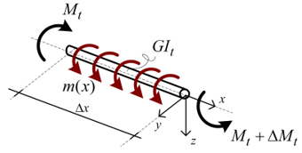
In this problem, all nodes only rotate around the \(y\)-axis; there’s no translation or rotation in another direction. For element \((3)\) and \((4)\) this introduces torsion in the elements. The model for torsional elements has been treated before in Week 2.2, Unit 2, Lecture 6 of this course [HansWfDUoTechnology24]:

Fig. 16 Torsional element from Hans Welleman from Delft University of Technology [HansWfDUoTechnology24]#
he differential equation for the this element can be derived leading to:
Kinematic relations: \(\theta=\cfrac{\mrm{d}\varphi_x}{\mrm{d}x}\)
Constitutive relation:\(M_t=GI_t \ \theta\)
Equilibrium relations: \(\cfrac{\mrm{d}M_t}{\mrm{d}x}=-m\)
These relations can be combined into one second order differential equation:
This looks identical (with \(m\) for \(q\), \(GI_t\) for \(EA\) and \(\varphi\) for \(u\)) to our results from the extension element, therefore, we can directly write down the stiffness matrix and (equivalent) force vector directly:
As our torsional elements \((3)\) and \((4)\) are identical, we get:
And for element \((4)\) an additional equivalent force vector due to the element load:
Reduce bending element for tractability#
Element \((1)\) and \((2)\) will bend in this case. However, no forces act in the local \(x\)-direction. This allows us to reduce the element defined in Local stiffness matrix Euler-Bernoulli element:
This gives for our numerical values:
Identify degrees of freedom#
As mentioned before, all nodes only rotate around the \(y\)-axis; there’s no translation or rotation in another direction. Therefore, the degrees of freedom are:
With \(\varphi\) being specifically \(\varphi_y\).
Assemble stiffness, element by element#
As all elements use the same orientation for the degrees of freedom, no transformation are required. Note that this requires:
Defining element \((1)\) from \(1\) to \(2\)
Defining element \((2)\) from \(2\) to \(3\)
Defining element \((3)\) from \(2\) to \(4\)
Defining element \((4)\) from \(3\) to \(5\)
Or all the other way around. Otherwise, the rotations at node \(2\) and \(3\) do not match.
Element \((1)\)#
The first element links the first and second nodal displacement with the first and second nodal forces:
Element \((2)\)#
The second element links the second and third nodal displacement with the second and third nodal forces:
Element \((3)\)#
The third element links the second and fourth nodal displacement with the second and fourth nodal forces:
Element \((4)\)#
The fourth element links the third and fifth nodal displacement with the third and fifth nodal forces:
Apply external loads#
Nodal loads#
Now, let’s add the external loads, starting with the nodal load at \(2\):
Equivalent nodal loads#
Let’s add the equivalent nodal loads from the continuous elements loads too:
Boundary loads#
And finally, let’s add the forces from the Neumann boundary conditions:
Complete system of equations#
Now, we found the complete system of equations:
Solving boundary conditions#
As we’ve no non-zero boundary conditions, we can apply the row-striking technique of lecture 1, which leads to:
Solving this system of equations gives:
\(\varphi_2 \approx 1 \cdot 10^{-4}\)
\(\varphi_3 \approx 1.6 \cdot 10^{-3}\)
The support reactions can be found by inserting these into our original system of equations and solving for the rows containing the support reactions:
Note that to calculate \(M_{t,4}\) the element load should be taken into account! This gives:
\(M_1 \approx 0.1 \text{ kNm}\)
\(M_{t,4} \approx -0.033 \text{ kNm}\)
\(M_{t,5} \approx -2.7 \text{ kNm}\)
Postprocessing moments element \(\left(1\right)\)#
The continuum displacement field of element \(\left(1\right)\) can be described by the shape function:
This gives:
This is a linear distribution, with values at \(x=0\) and \(x=\ell\):
\(M \left(0\right) \approx -0.1 \text{ kNm}\)
\(M \left(2\right) \approx 0.2 { kNm} \)
The value at \(x=0\) has indeed the same absolute value as the support reactions. The sign is different because \(M_1\) is defined in the global coordinate system and \(M \left(0\right)\) is defined from our agreements on positive internal moments (leading to positive stresses at the positive \(z\)-side.)
